Graphing a Linear Equation as a Transformation of the Parent Function

Graphing Transformations of the Parent Function

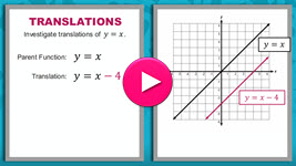Get ready to extend your knowledge of translations, reflections, and dilations. In this interactivity, you will learn how to apply these transformations to the graph of the simplest linear equation, the linear parent function y = x. Click the player button to begin.

View a printable version of the interactivity.

 

 

Graphing a Line as a Transformation of the Parent Function

Example: Graph the linear parent function after the following transformations:

• a translation 1 unit down; and
  
• a compression by a factor of
  2/5
  .

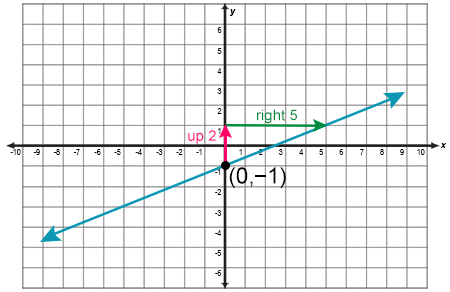
Explanation

Step 1: Begin by addressing the translation first, since this transformation affects the y-intercept.

Since you are told that the graph of the parent function has been translated 1 unit down, you know that the y-intercept is −1. Plot the y-intercept (0, −1).

Step 2: Now, move on to the compression.

The compression by a factor of 2/5 informs you that the slope has been changed to 2/5.

So, begin at the y-intercept and rise up 2 units and move right 5 units. The point where you end is another point on the line (5, 1). Draw a line that passes through the two points.

 

Graphing a Linear Equation as a Transformation of the Parent Function Review

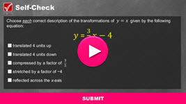
Now that you have explored graphing a linear equation as a transformation of the parent function, it is time to review your knowledge and practice what you have learned. Click the player button to get started.

 

 

 

Did you answer the content review questions incorrectly? Do you want more instruction or extra practice? If so, view the video Graphing a Line by Using Transformations of the Parent Function from eMediaVASM.